Composing multiple plots with patchwork
patchwork
It’s often useful to compose multiple plots together into a single image. There are ways of doing this in base R, e.g., by using par(mfrow=...), but i’ve always found this unintuitive and finicky. patchwork makes composing ggplots simple, while allowing for a high degree of customization. (The patchwork documentation is very good, and this post will borrow liberally from it, but it’s worth browsing for more details.) (For those looking for an alternative to patchwork, check out cowplot::plot_grid().)
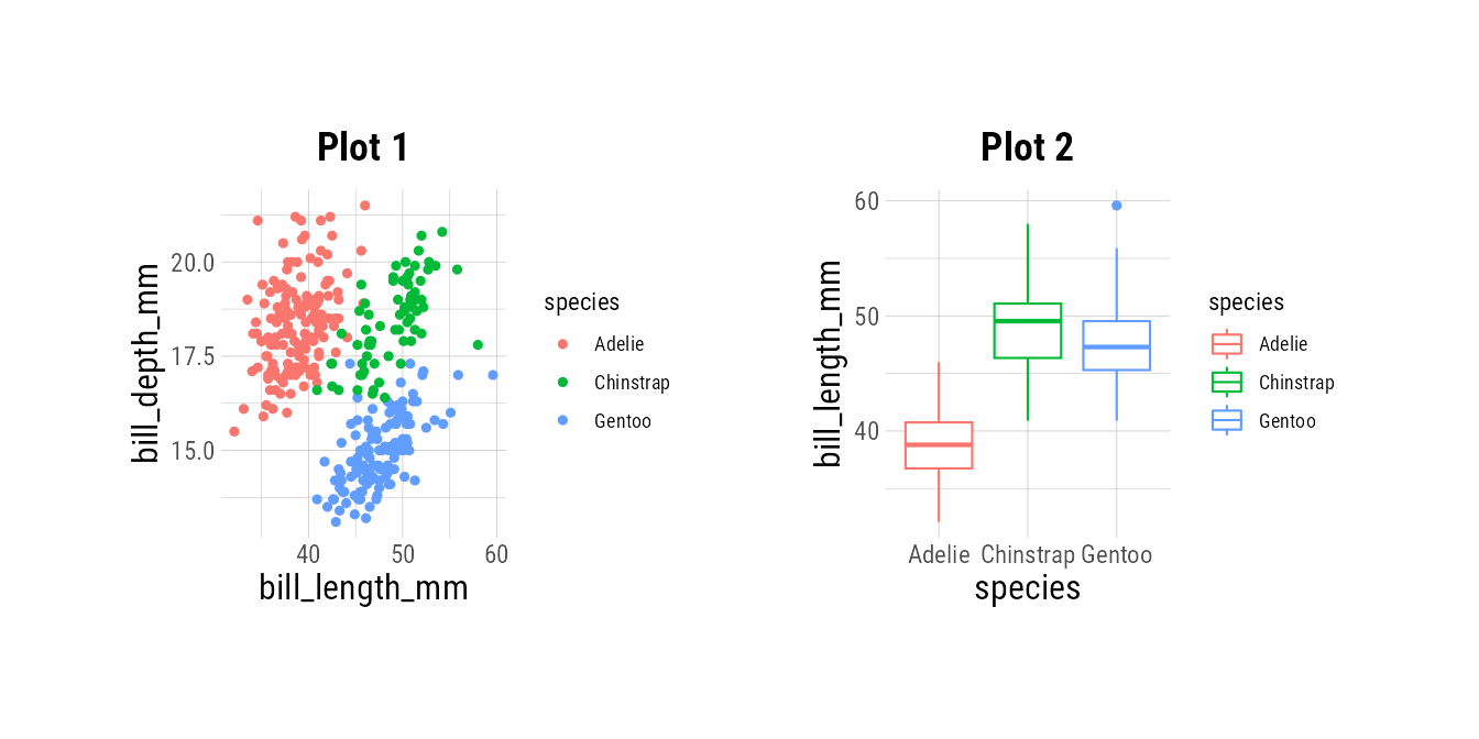
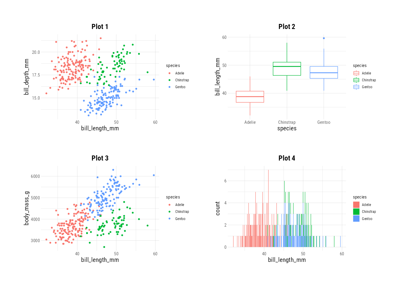
Let’s start with 4 simple plots, and look at various ways of composing them. (These plots are nicely arranged in a grid by Quarto for the purposes of this page if your browser window is big enough, but note that they are each a separate image.)
Code
p1 <- ggplot(palmerpenguins::penguins) +
geom_point(aes(bill_length_mm, bill_depth_mm,
color = species)) +
ggtitle("Plot 1")
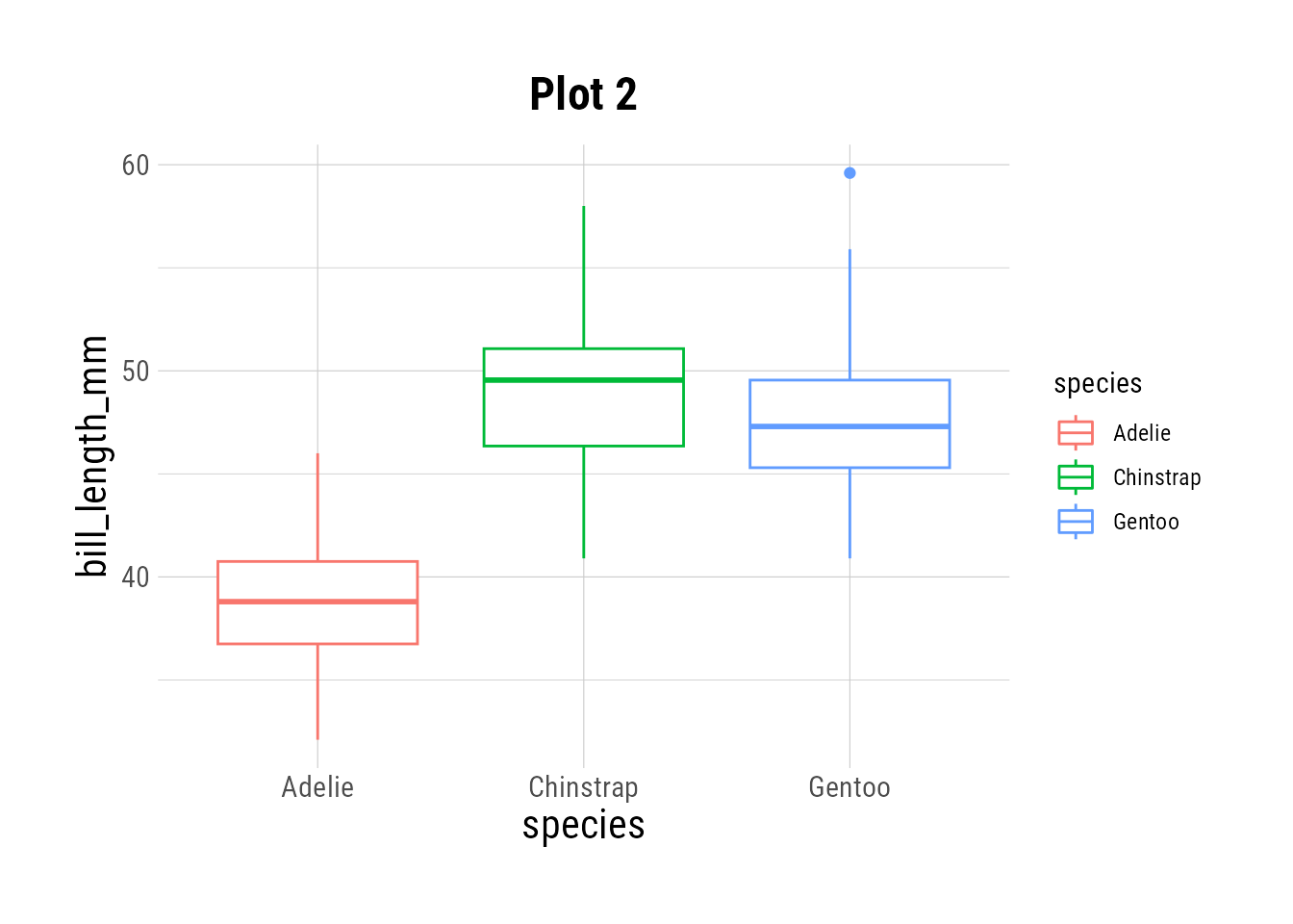
p2 <- ggplot(palmerpenguins::penguins) +
geom_boxplot(aes(y = bill_length_mm, species,
color = species)) +
ggtitle("Plot 2")
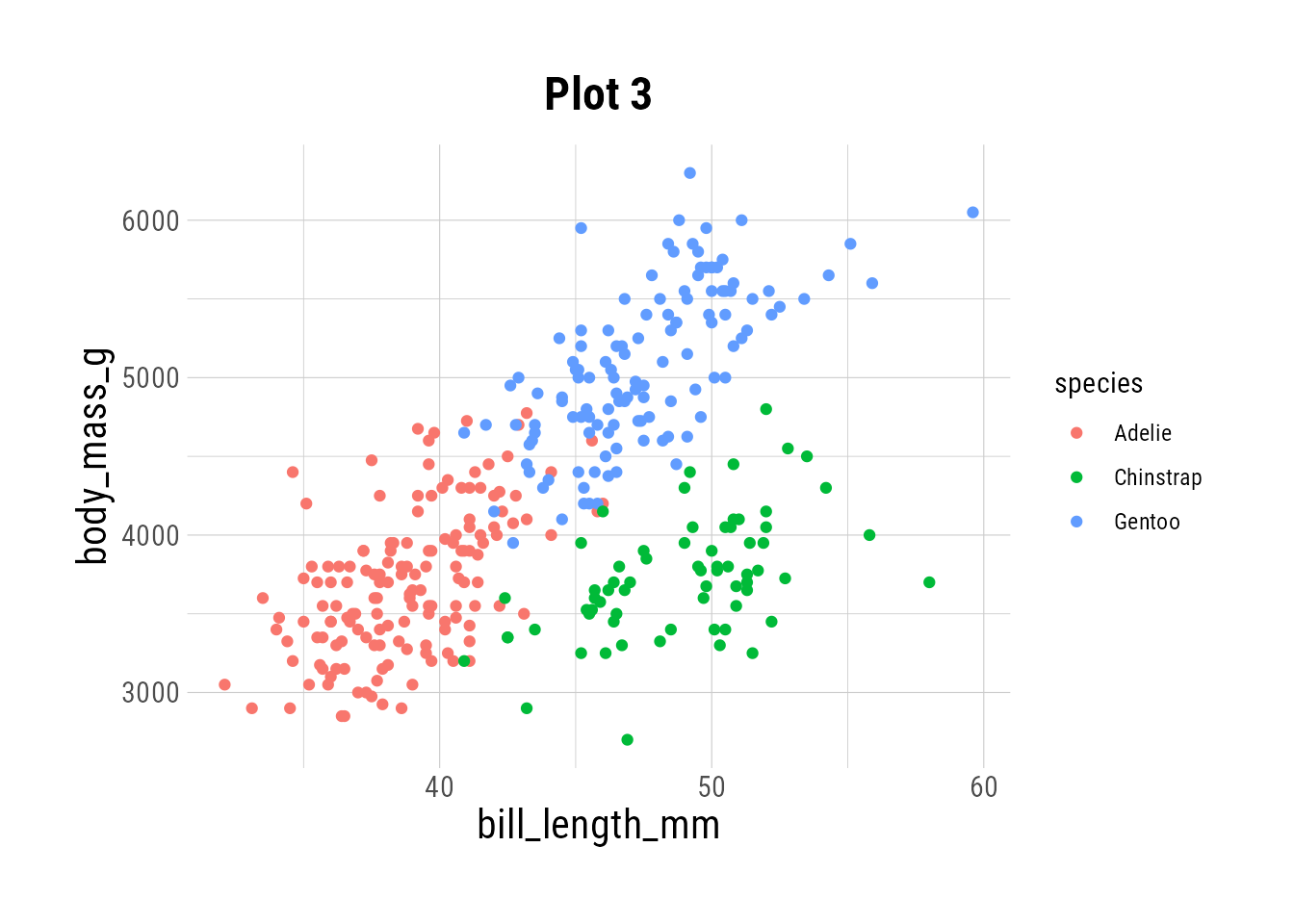
p3 <- ggplot(palmerpenguins::penguins) +
geom_point(aes(bill_length_mm, body_mass_g,
color = species)) +
ggtitle("Plot 3")
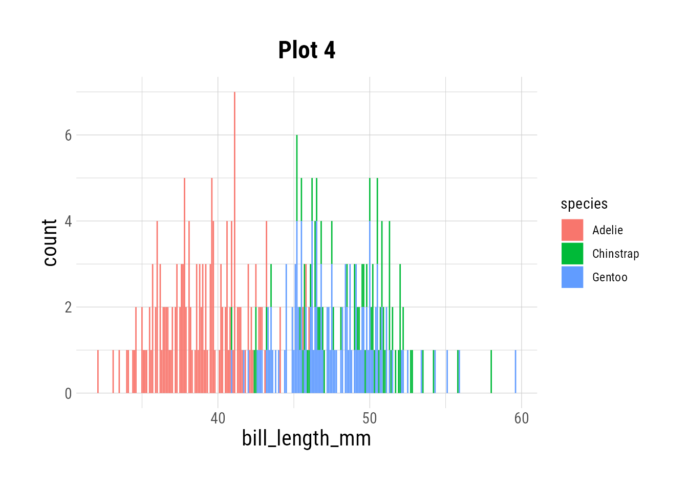
p4 <- ggplot(palmerpenguins::penguins) +
geom_bar(aes(bill_length_mm, fill = species)) +
ggtitle("Plot 4")
p1; p2; p3; p4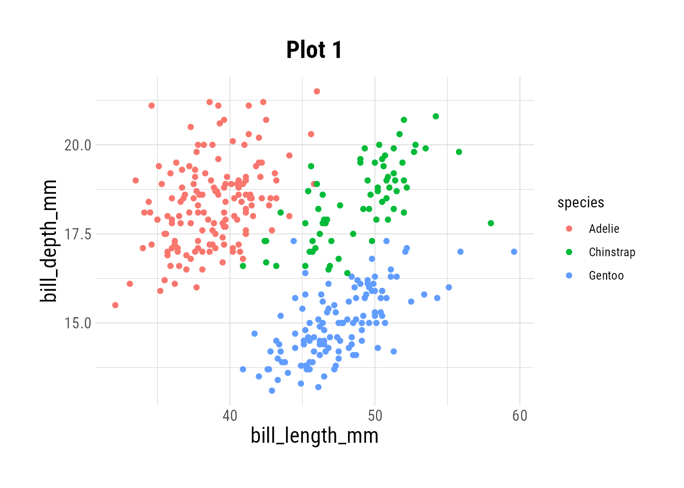
The simplest operation provided by patchwork is the + operator. Adding two plots together with + glues them together into a single image, side by side. You can do this with as many plots as you like–it will try to give a nice grid if possible. Note that all plots below are combined into a single image.
You can specify the number of rows or columns in your composed plot with plot_layout(nrow=..., ncol=...). Setting byrow to false fills by column, rather than by row (so the left column below has plots 1, 2, and 3). (Click image to embiggen.)
p1 + p2 + p3 + p4 +
  plot_layout(nrow = 3, byrow = FALSE)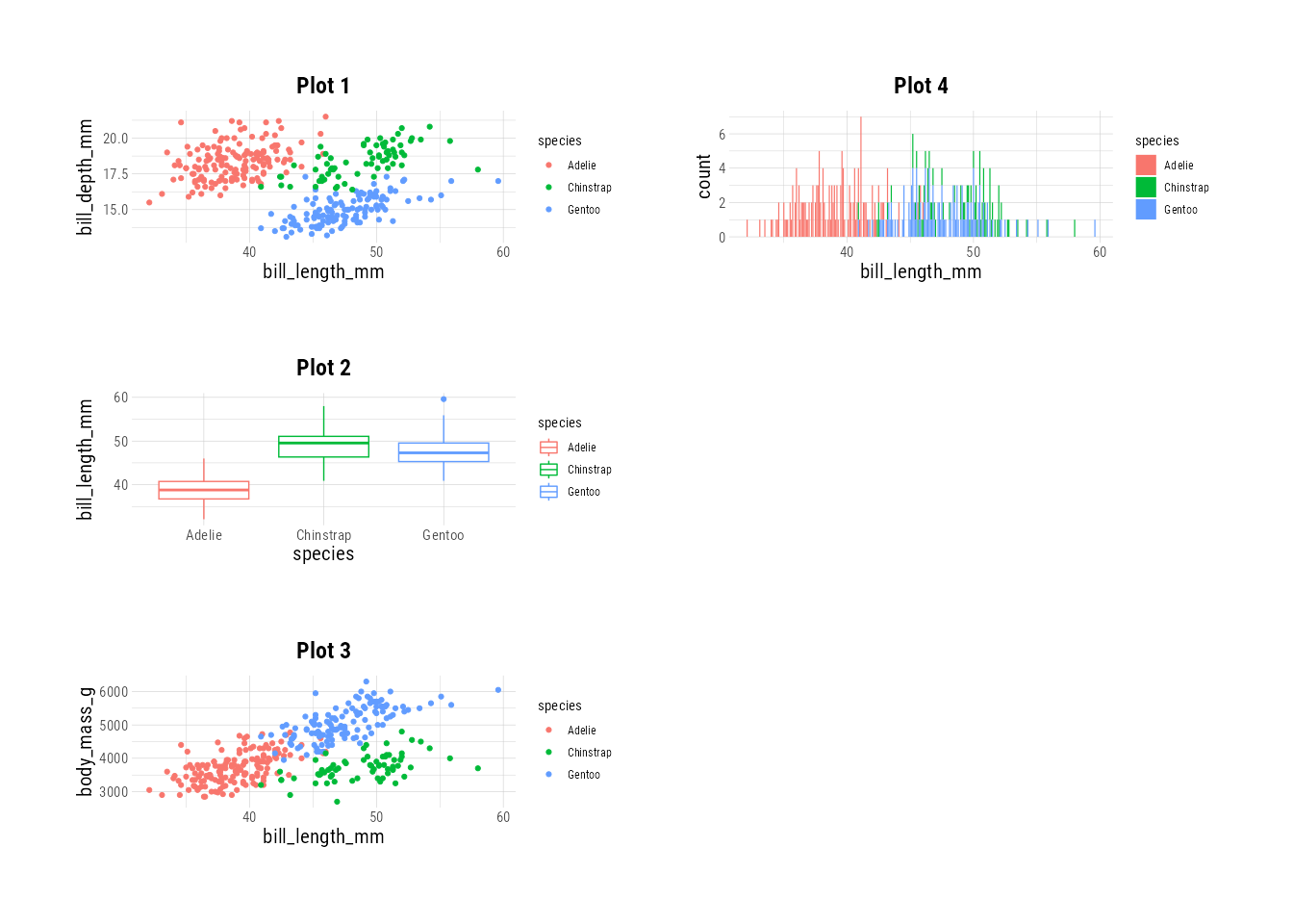
See the section below on more complicated layouts and ?plot_layout for more options.
Packing and stacking (the | and / operators)
Composing two plots with the | operator works a lot like the + operator above, except it ensures that the plots will end up side-by-side (“packed”) rather than one on top of the other. The / operator does the opposite—it ensures that plots are stacked.”
p1 | p2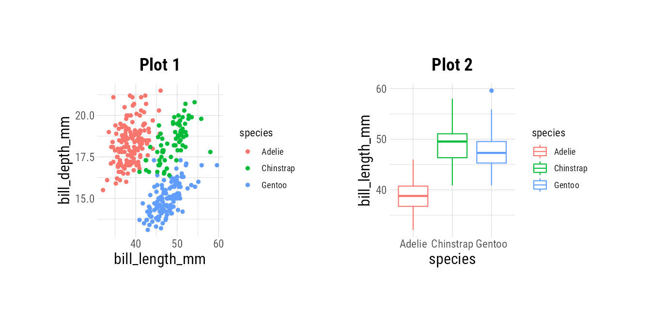
p1 / p2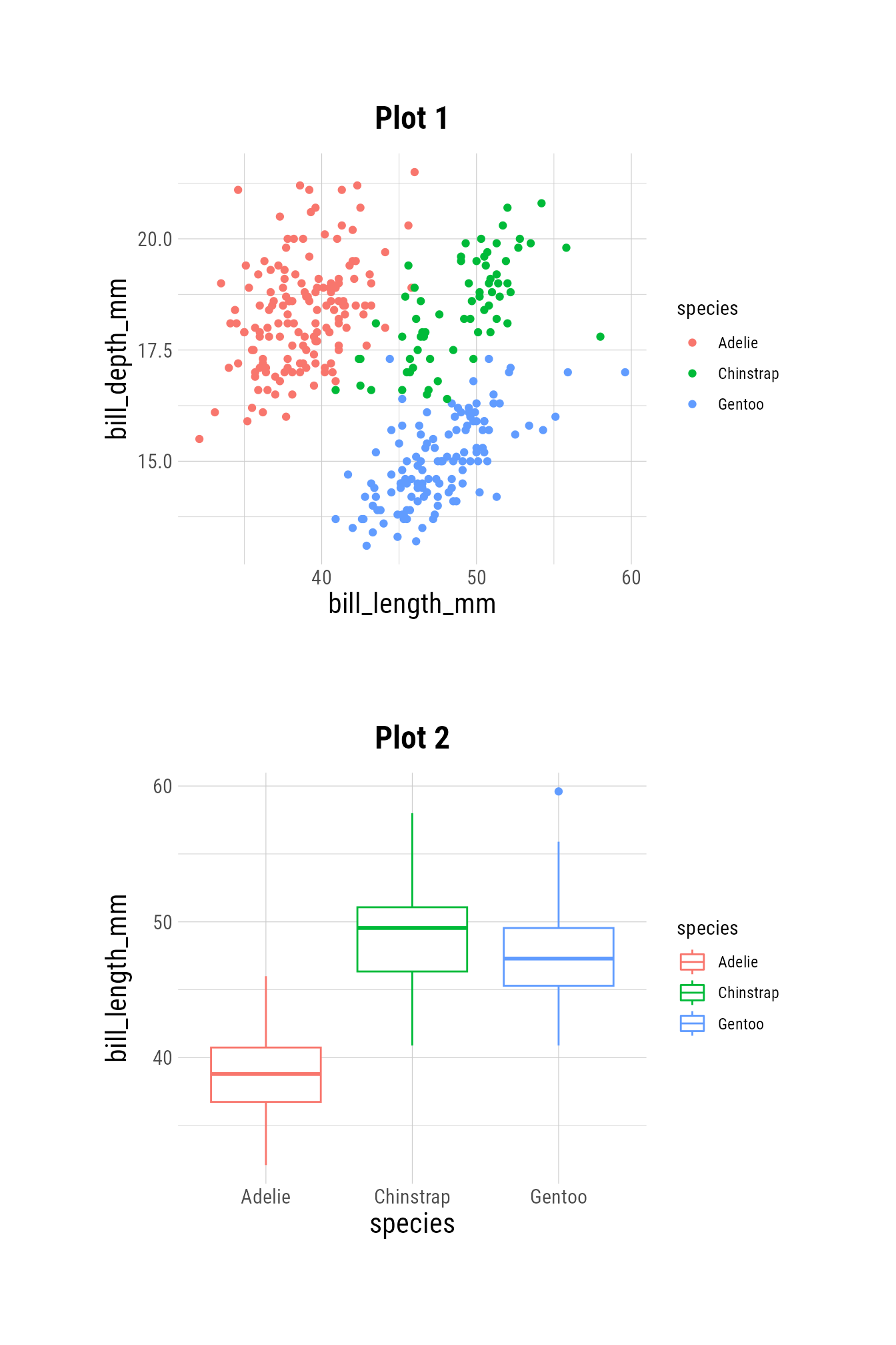
Parentheses can help to disambiguate possible layouts. (All of the operators work essentially like their arithmetic counterparts with respect to parentheses.) Without parentheses, as in the first tab below, the / operator takes precedence over the | operator:
p1 / p2 | p3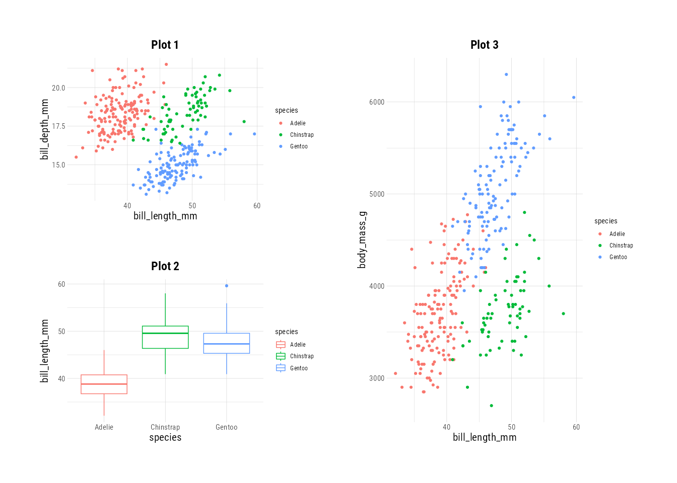
p1 / (p2 | p3)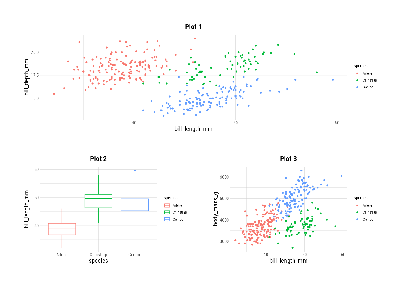
Annotating the composed plot
plot_annotation() will annotate the combined, composed plot. The title and subtitle, arguments work as you would expect. The tag_levels argument lets you specify one of c('a', 'A', '1', 'i', 'I') for various sub-plot numbering:
(p1 | (p2 / p3)) +
  plot_annotation(title = 'Lots of data about penguins',
    subtitle = 'There\'s never too much info about penguins',
    tag_levels = "A") &
  theme(plot.title = element_text(hjust = .5, color = "blue"),
        plot.tag = element_text(size = 20))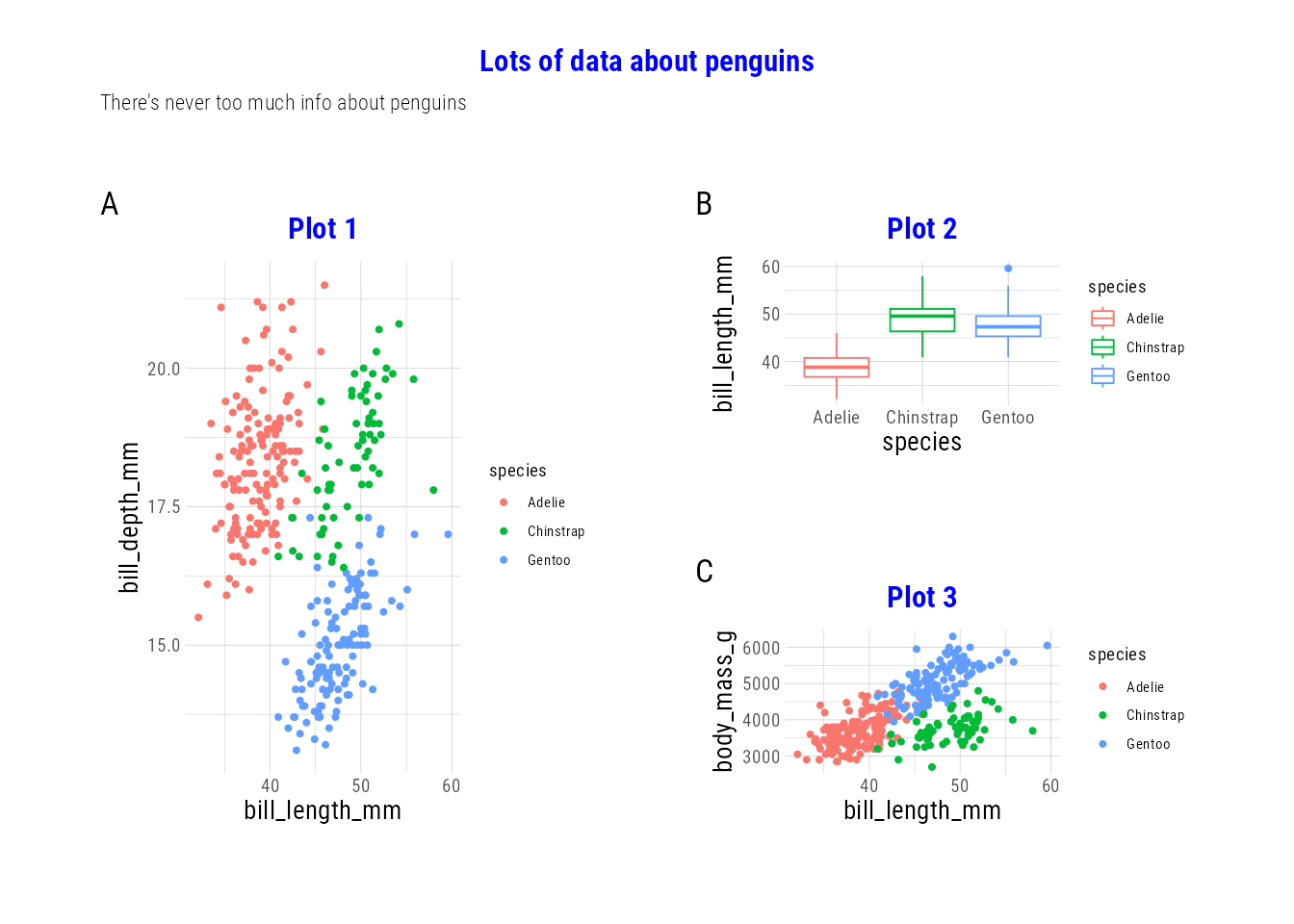
(The & operator applies the theme specification to all subplots within the composed plot (and overall things like the main title/subtitle); the * operator applies the theme specifications to all subplots in the current nesting. level.)
If you want a theme element to apply only to the overall plot, and not the subplots, use the theme argument to plot_annotation() rather than & theme(...).
(p1 | (p2 / p3)) +
  plot_annotation(title = 'Lots of data about penguins',
    subtitle = 'There\'s never too much info about penguins', tag_levels = "A",
    theme = theme(plot.title = element_text(hjust = .5, color = "blue"),
        plot.tag = element_text(size = 20)))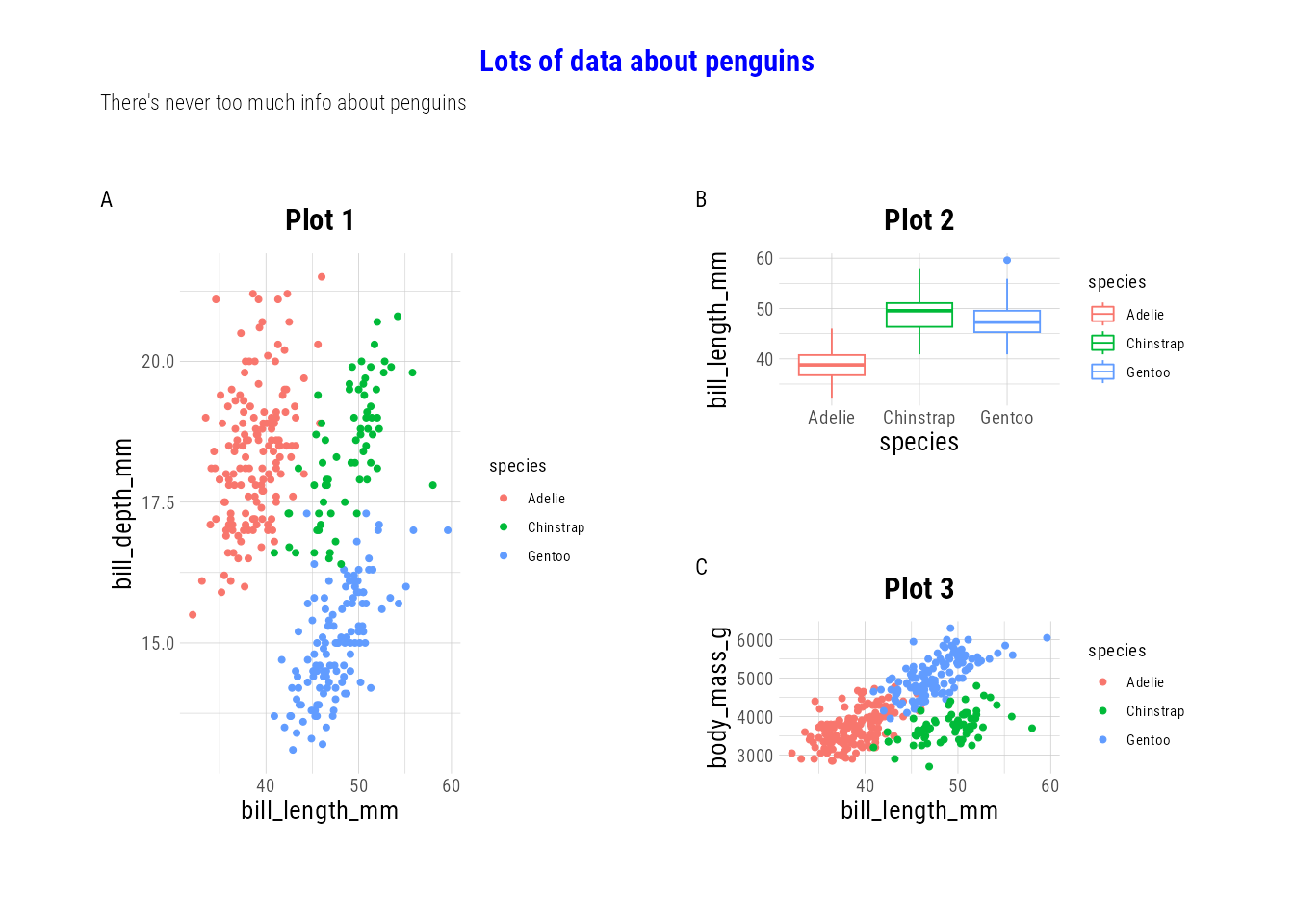
More complicated layouts
We saw above that we can modify the layout with plot_layout(ncol = ...). You can also specify relative widths and heights for the rows and columns. For example, you can provide widths with a vector of n columns to specify each.
Some plot theme changes for visibility in the following examples
p1 <- p1 + theme(legend.position = "none", plot.background = element_rect(color = "black", linewidth = 2, fill = "white"))
p2 <- p2 + theme(legend.position = "none", plot.background = element_rect(color = "blue", linewidth = 2, fill = "white"))
p3 <- p3 + theme(legend.position = "none", plot.background = element_rect(color = "green", linewidth = 2, fill = "white"))
p4 <- p4 + theme(legend.position = "none", plot.background = element_rect(color = "red", linewidth = 2, fill = "white"))
p1 + p2 + p3 + p4 +
plot_layout(widths = c(3, 1), heights = c(2, 1))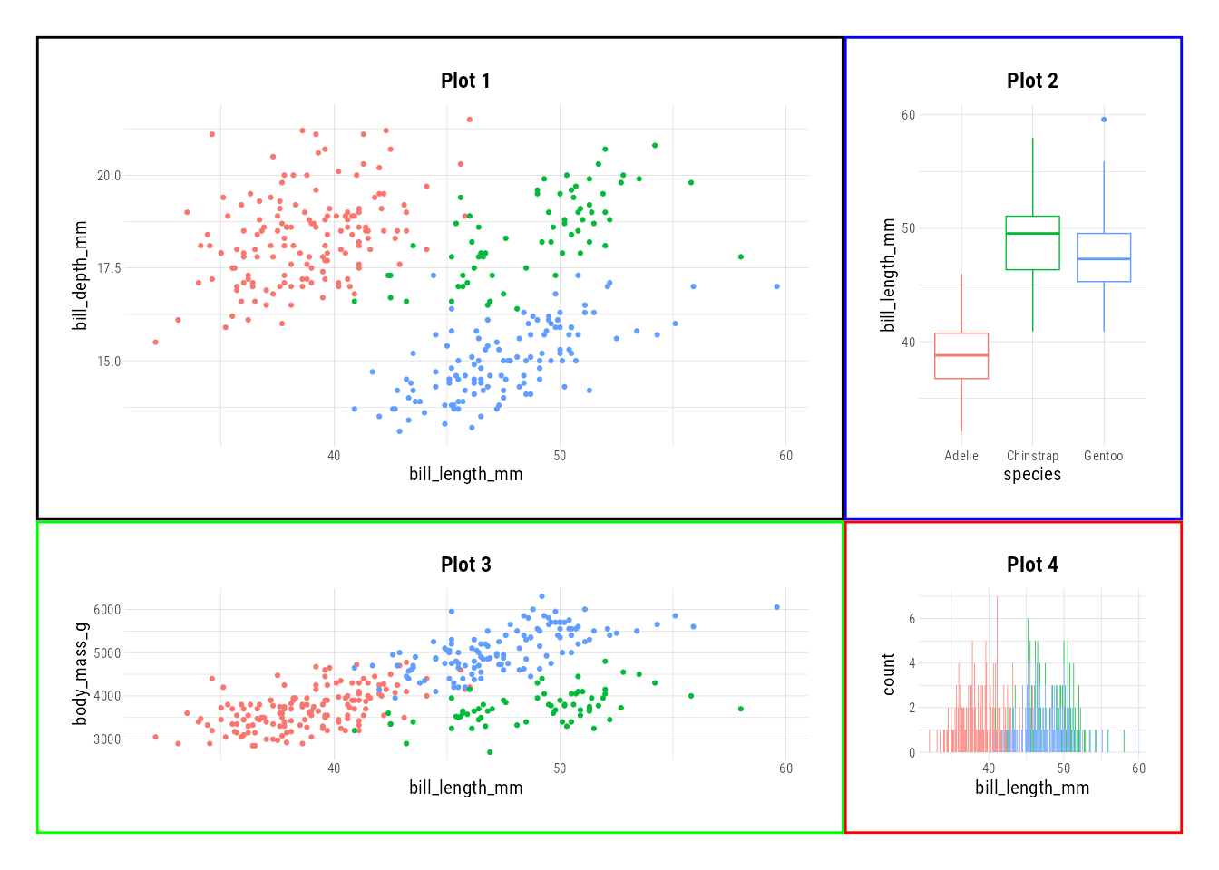
You can also specify quite complicated layouts with plot_layout(design = ...), in two formats. The simplest is to use a textual representation, as below. Letters represent plots (in the order in which they appear), with #s representing empty spaces. You must specify a perfect rectangular shape.
layout <- "
##BBBB
AACCDD
##CCDD
"
p1 + p2 + p3 + p4 +
  plot_layout(design = layout)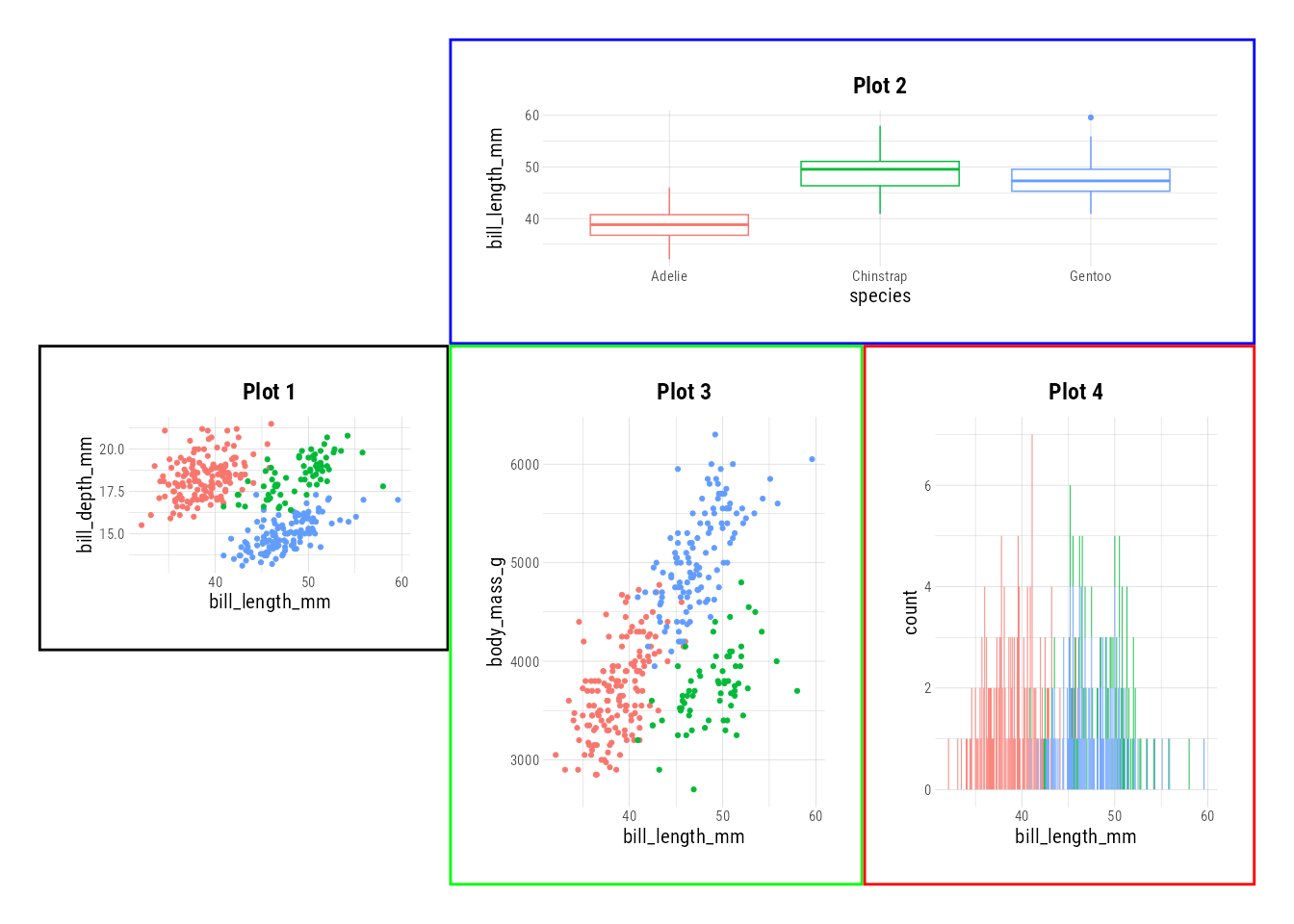
Using wrap_plots, you can specify which plot is represented by which letter, rather than letting that be handled automatically:
layout <- '
A#B
#C#
D#E
'
wrap_plots(D = p1, C = p2, B = p3, design = layout)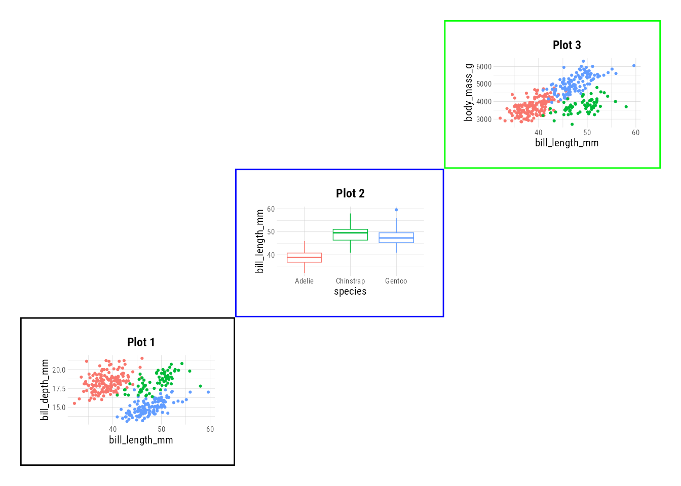
The alternative way to specify a layout is with one or more area()s, which take arguments for the top, left, bottom, and right bounds of a grid.1 The grid is specified in rows and columns, with row 1 column 1 being the top left, and numbers increasing as you go down and right. You can have plots overlap with this type of specification.
layout <- c(
  area(t = 2, l = 1, b = 5, r = 4), # This will be p1
  area(t = 1, l = 3, b = 3, r = 5) # this will be p2
)
p1 + p2 +
  plot_layout(design = layout)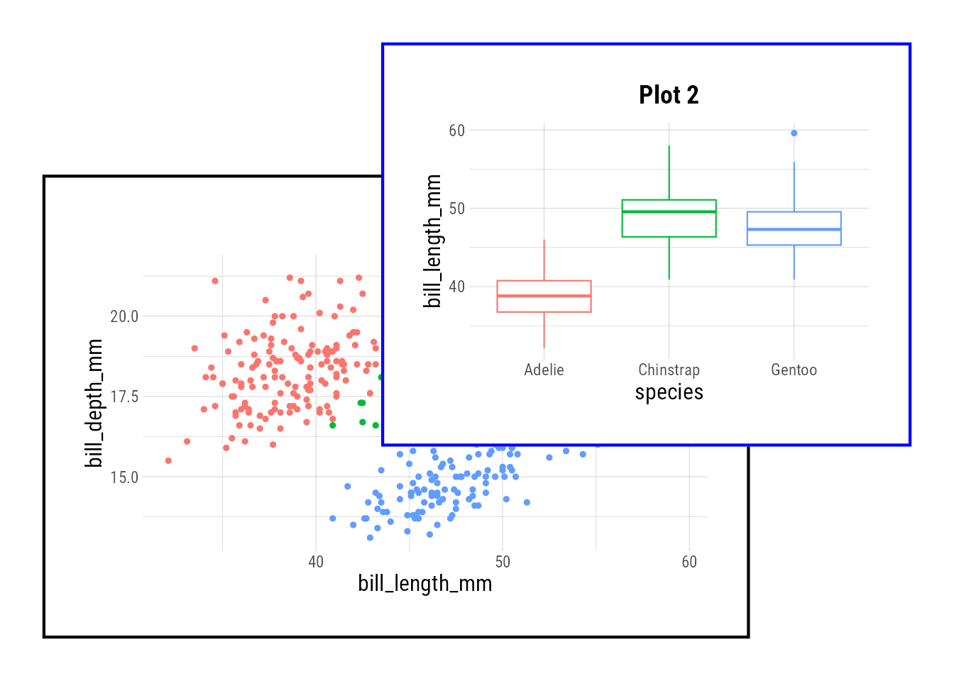
Insets
It’s also possible to specify insets using inset_element(). Here, the position arguments should be relative to 1, with (0, 0) being bottom left and (1, 1) being top right. The align_to argument defaults to panel, but accepts values plot or full as well.
p1 + inset_element(p2, top = 1, right = 1, bottom = .5,
                   left = .5, align_to = "full")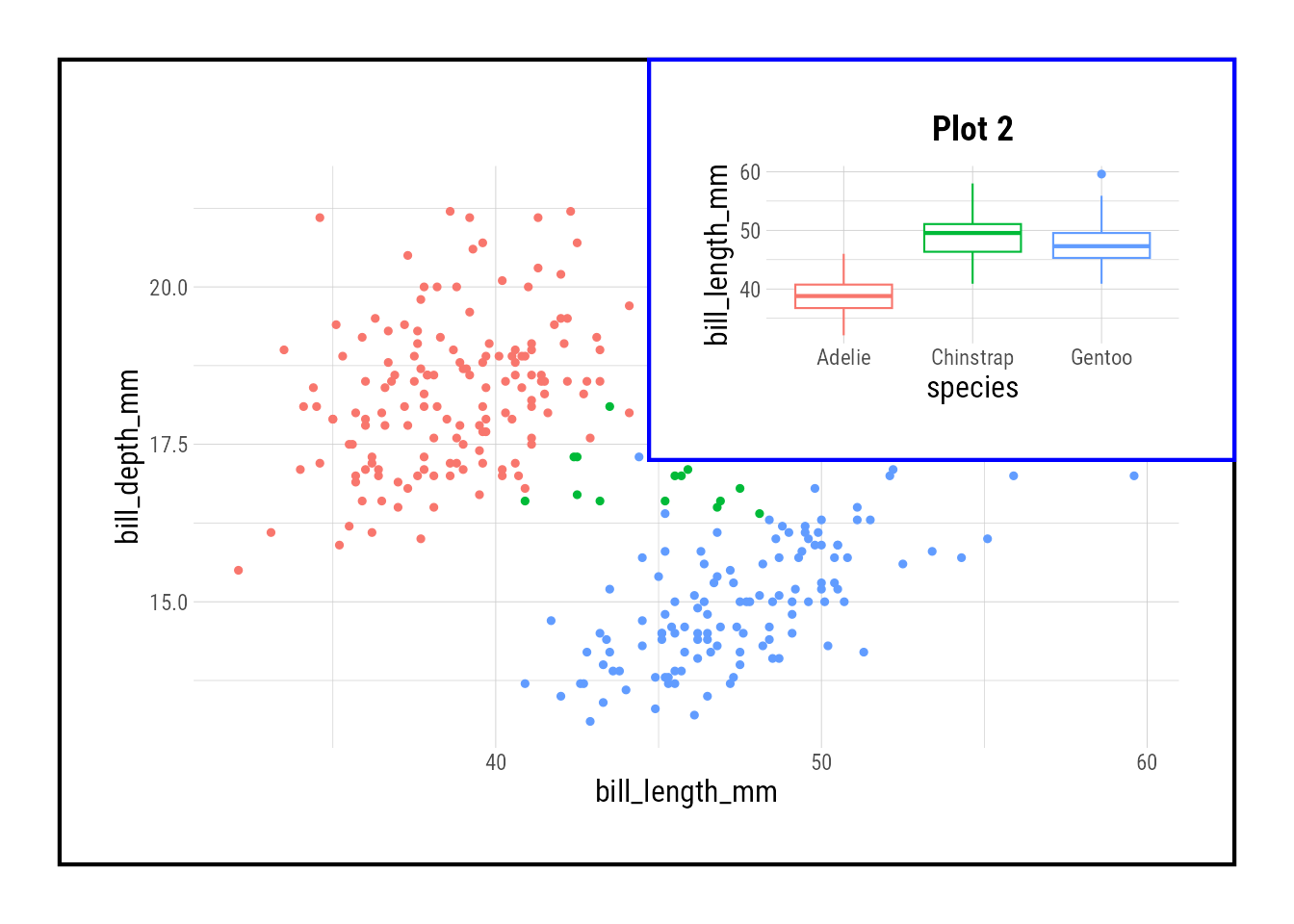
Controlling legends
Reset plots to their original theme
p1 <- p1 + theme(legend.position = "right", plot.background = element_blank())
p2 <- p2 + theme(legend.position = "right", plot.background = element_blank())
p3 <- p3 + theme(legend.position = "right", plot.background = element_blank())
p4 <- p4 + theme(legend.position = "right", plot.background = element_blank())
plot_layout(guides = "collect") will collect all of the legends and put them in the same location. Legends that are identical between multiple subplots are collapsed, as with plots 1 and 3 below:
p1 + p2 + p3 + p4 + plot_layout(guides = "collect")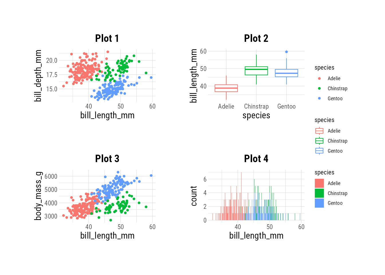
p1 + p2 + p3 + p4 + plot_layout(guides = "keep")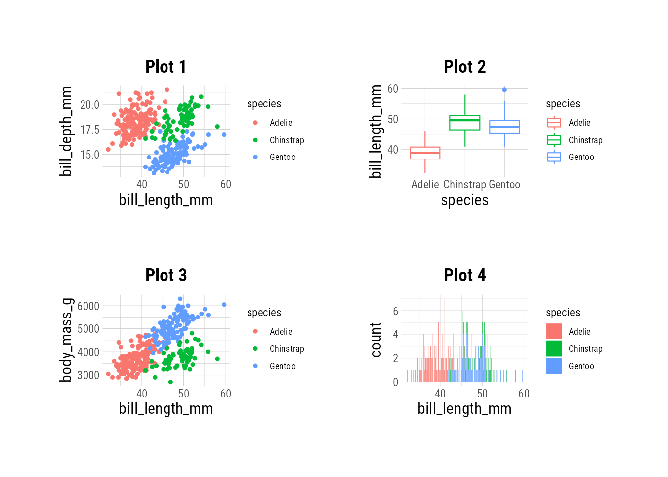
You can influence where the collected legends show up by including guide_area() in your layout specification:
guide_area() + p1 + p2 + p3 + plot_layout(guides = "collect")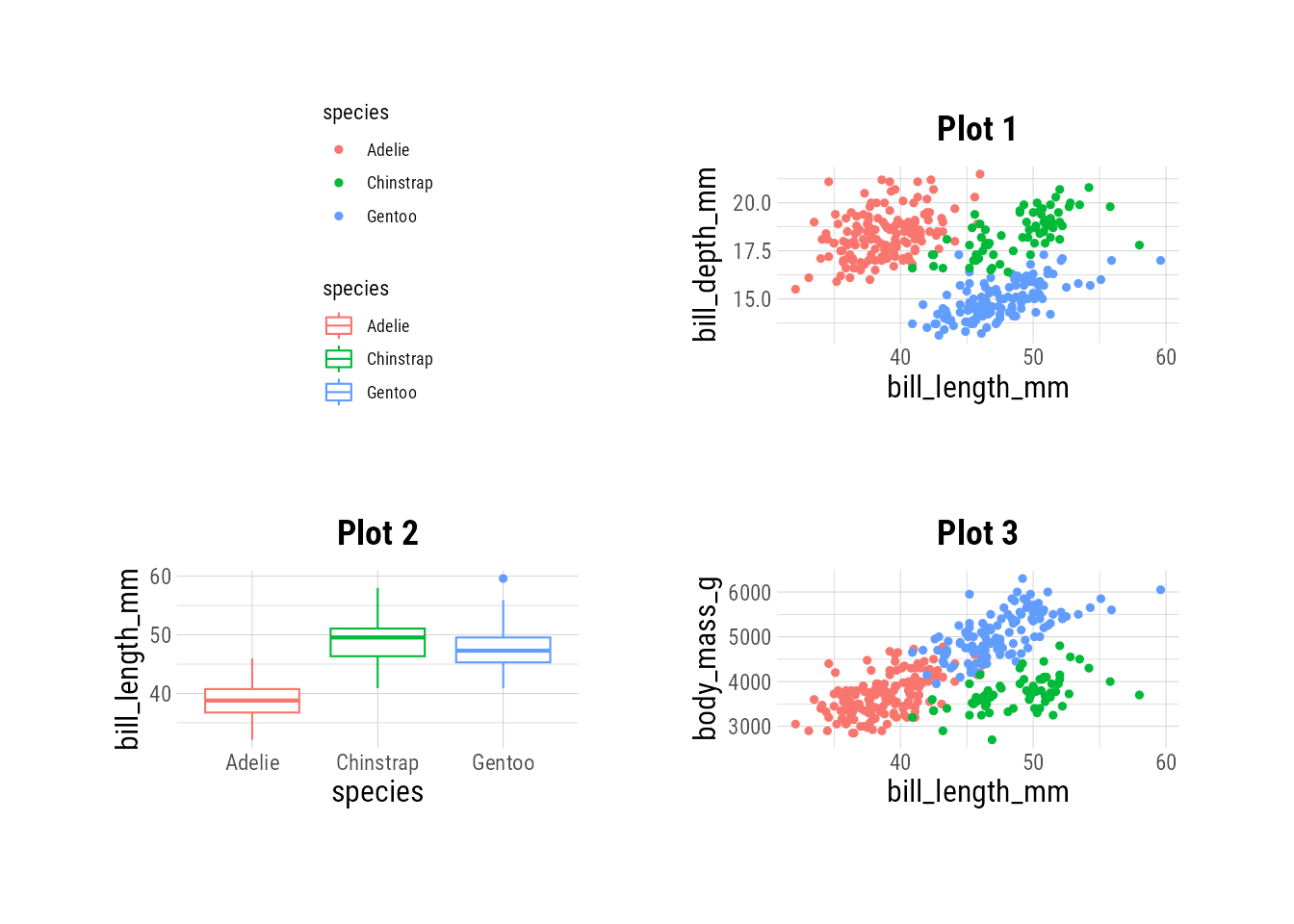
Nesting
Some plot theme changes for visibility in the following examples
p1 <- p1 + theme(legend.position = "none", plot.background = element_rect(color = "black", linewidth = 2, fill = "white"))
p2 <- p2 + theme(legend.position = "none", plot.background = element_rect(color = "blue", linewidth = 2, fill = "white"))
p3 <- p3 + theme(legend.position = "none", plot.background = element_rect(color = "green", linewidth = 2, fill = "white"))
p4 <- p4 + theme(legend.position = "none", plot.background = element_rect(color = "red", linewidth = 2, fill = "white"))
Plots can be nested at multiple levels. Compare the following plots: in the first we use wrap_plots() to combine p1 and p2 into a single unit (which is then added to plot 3); in the second we don’t do any nesting.
wrap_plots(p1 + p2) + p3
(p1 + p2) + p3 # Parens are vacuous here
If you don’t use wrap_plots(), the nesting behavior with + is a little unintuitive. With a single plot on the left of + and a composite plot on the right, you get the expected nesting, with the composite plot taking up half of the whole plot:
composite <- p1 + p2
p3 + composite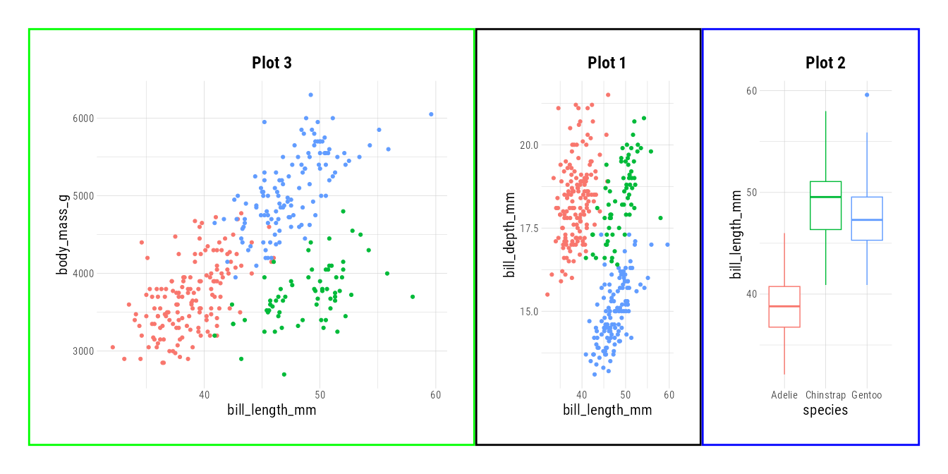
So far, so good. But, what if we change the order of arguments around +? All of a sudden, the plot is divided into 3 equal panels!
composite + p3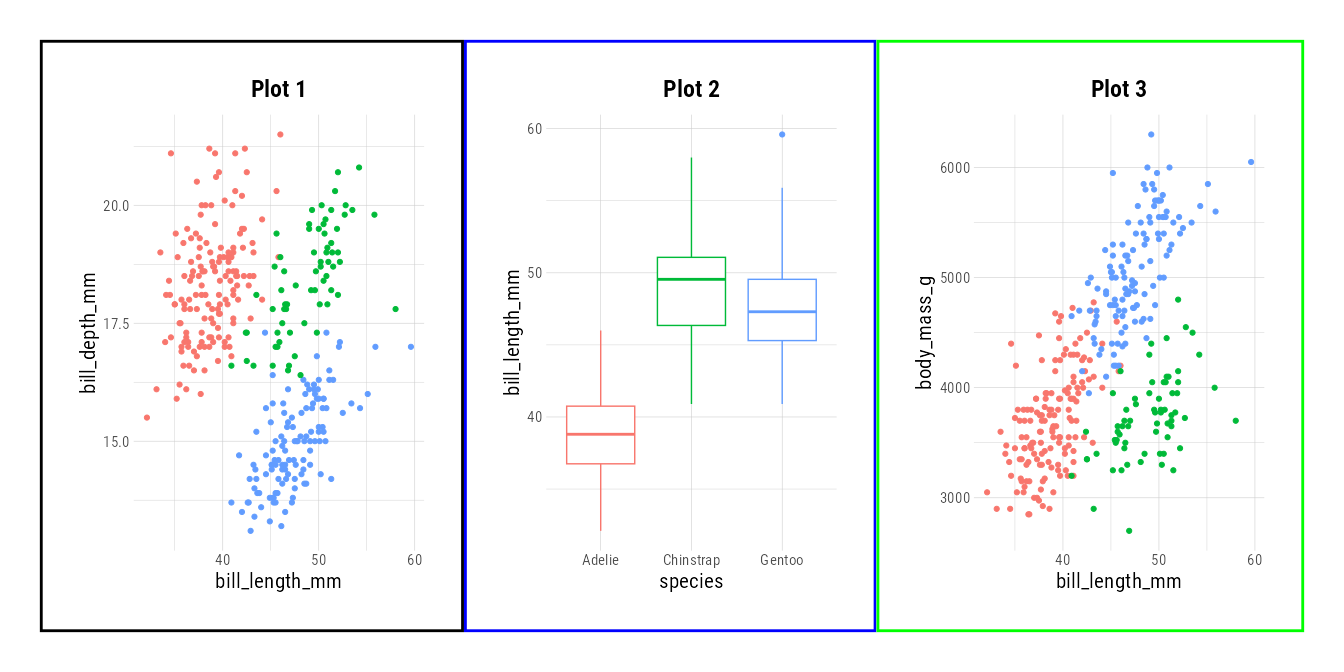
So, + will nest a composite on the right, but will not nest a composite on the left. You can force the reverse of this by using the - operator, which keeps its arguments at the same nesting level—but I personally find the wrap_plots() syntax more intuitive.
composite - p3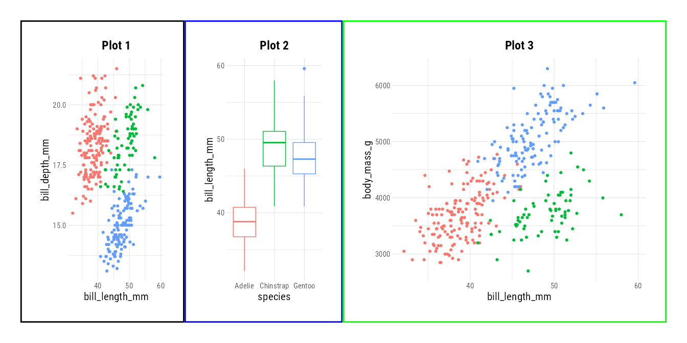
p3 - composite
Alignment across multiple slides
Some plot theme changes for visibility in the following examples
p1 <- p1 + theme(legend.position = "top", plot.background = element_blank())
p2 <- p2 + theme(legend.position = "right", plot.background = element_blank())
p3 <- p3 + theme(legend.position = "bottom", plot.background = element_blank())
p4 <- p4 + theme(legend.position = "left", plot.background = element_blank())
When including plots in a slideshow, you often get an annoying jerking sensation as you move from one slide to the next:
You can generate aligned plots align_patches. Notice here how the axis labels are aligned with each other across multiple slides.
plots_aligned <- align_patches(p1, p2, p3, p4)
for (p in plots_aligned) {
  plot(p)
}
See the relevant documentation for more details.
Footnotes
Somewhat annoyingly, the argument order here is
tlbr, rather thantrblas in css, which is how my brain works.↩︎