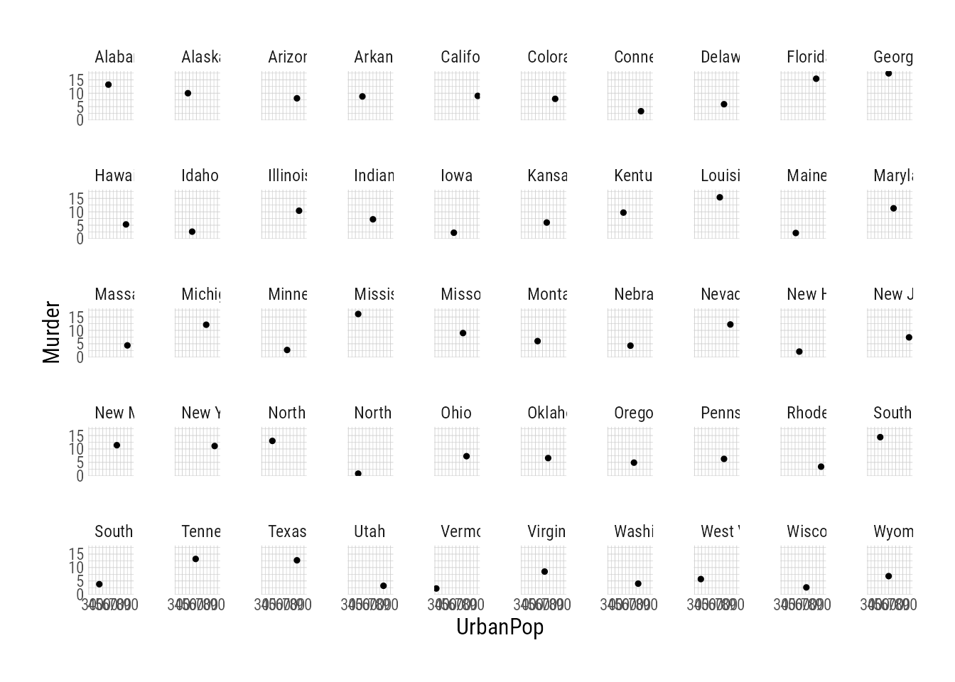
When you have a plot with just a few facets, it’s easy to fit them all on a single page. But what if you have a whole bunch of facets that you want to visualize? For example, the USArrests dataset has data from all 50 US states.
If we just use the usual facet_wrap or facet_grid from ggplot2, you end up with one massive, smooshed-together image:
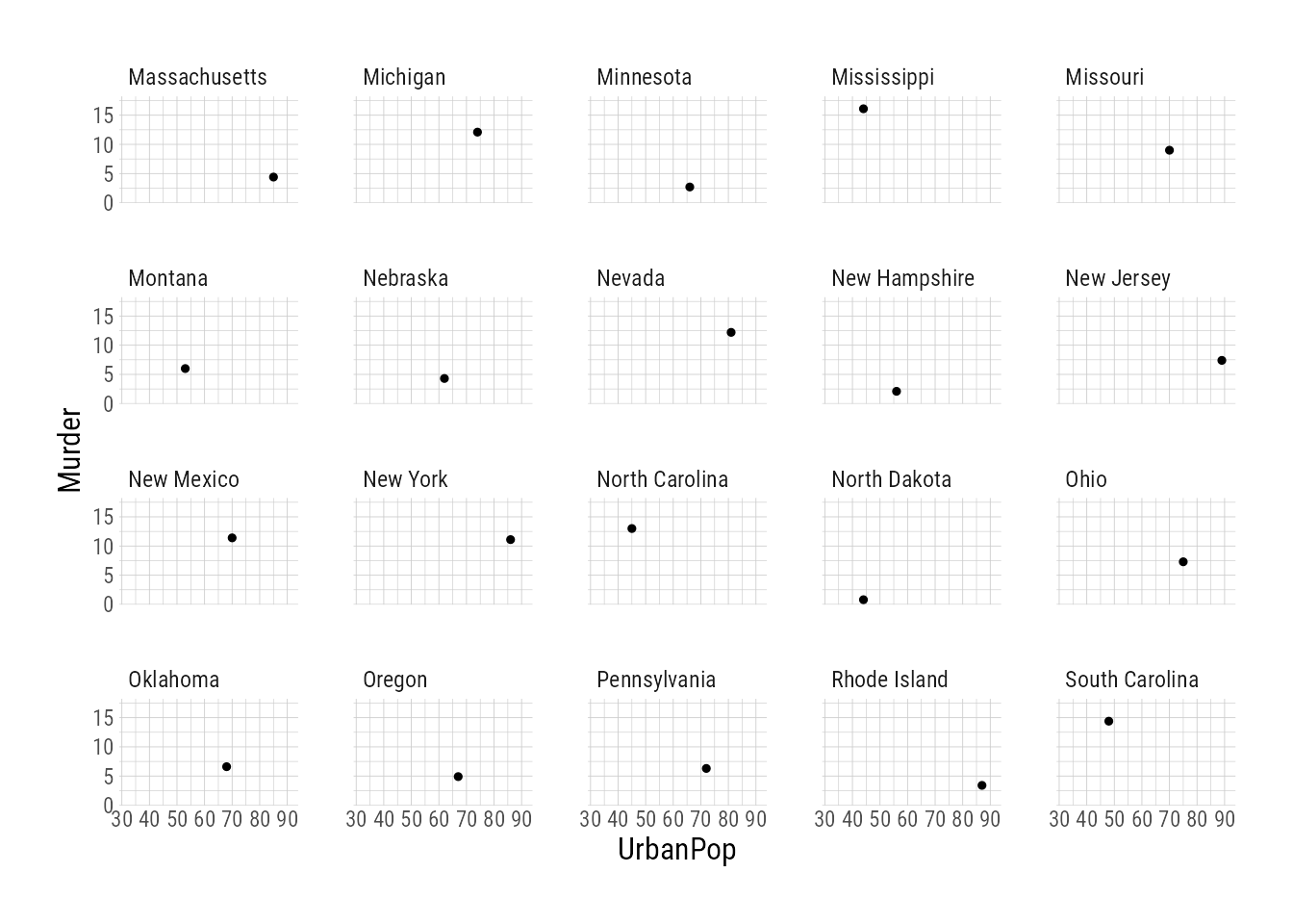
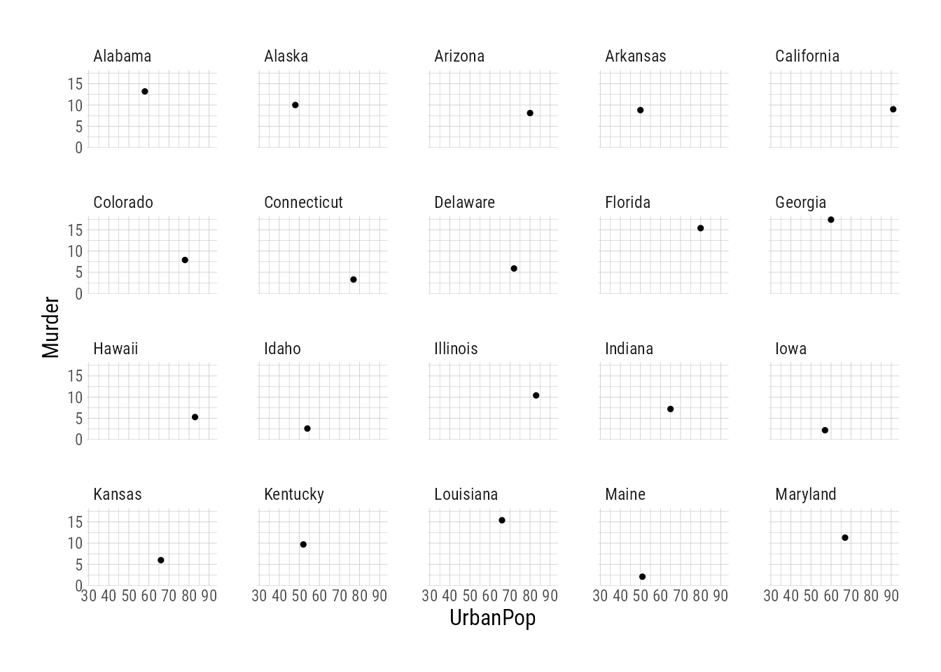
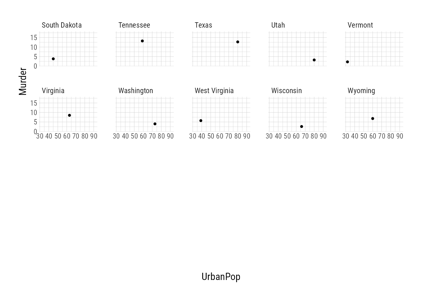
The ggforce library, among its many useful functions, includes facet_wrap_paginate and facet_grid_paginate. These work like facet_wrap and facet_grid, but take an additional page argument. Here we specify that we want 4 rows and 5 columns per page, so for 50 states there will be 2 full pages plus one page with the remaining 10 states:
Note that we had to specify which page we wanted to print. We can then easily put this into a loop to generate all the necessary pages. The helpful n_pages() will count the pages needed, which we can then use in a loop. This gives us 3 separate plots.
That’s better, but for inclusion in a longer document or for sharing the plot, you may want all three pages in a single PDF. This can be accomplished by calling pdf() before the loop and dev.off() after.1
pdf('many_plots.pdf', width =11, height =8.5)#start building pdffor(iin1:plot_pages){print(# don't forget thisplot_1+facet_wrap_paginate(~State, nrow =4, ncol =5, page =i))}dev.off()# end building pdf
The resulting PDF is a single file with 3 pages, as we expect.
In the past I’ve had issues with getting pdf() to work, especially if I use any fancy fonts in the ggplot theme. If you run into issues, you can replace pdf() with cairo_pdf(..., onefile = TRUE), which seems to work even with exotic fonts.↩︎